Part 4 of the 600,000 Questions benchmark series
TL;DR
Testing vLLM with 1, 4, and 16 concurrent queries revealed near-linear scaling for throughput with zero accuracy loss. MMLU wall-clock time dropped from 7.1 minutes (sequential) to 1.5 minutes (16 parallel)—a 4.7x speedup. GSM8K scaled even better: 78.7 minutes down to 8.6 minutes (9.2x speedup). The key insight: vLLM’s continuous batching handles concurrent requests efficiently, making parallelism essentially free for throughput-bound workloads. If you’re running batch inference, you’re leaving performance on the table by processing sequentially.
The previous parts of this series focused on model selection—which architecture, which quantization level, which size. But there’s another dimension to inference performance that gets surprisingly little attention: how many requests should you send at once?
Sequential processing is the default for most benchmarking. Send a question, wait for the answer, record the time, repeat. It’s simple, it’s predictable, and it completely misses how production systems actually work.
vLLM’s architecture is built around continuous batching—the ability to dynamically group incoming requests and process them together on the GPU. In theory, this should allow multiple concurrent requests to share compute resources efficiently. In practice, the question is: how much speedup do you actually get, and does accuracy suffer?
I ran the full MMLU and GSM8K benchmarks at three parallelism levels to find out.
The Experiment
Same model throughout: Qwen3-VL-30B with AWQ 4-bit quantization, running on vLLM. Same 14,042 MMLU questions and 1,319 GSM8K questions. The only variable: how many requests were in flight simultaneously.
- Parallel=1: Sequential baseline. One request at a time.
- Parallel=4: Modest concurrency. Typical for a small application.
- Parallel=16: Aggressive batching. Stress-testing the system.
MMLU Results: Throughput Scales, Accuracy Doesn’t Budge
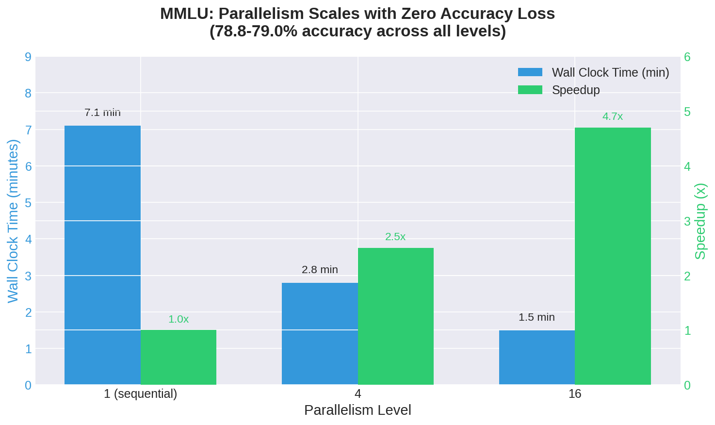
| Parallelism | Accuracy | Avg Time/Question | Wall Clock Time | Speedup |
|---|---|---|---|---|
| 1 | 78.9% | 0.030s | 7.1 min | baseline |
| 4 | 79.0% | 0.047s | 2.8 min | 2.5x |
| 16 | 78.8% | 0.101s | 1.5 min | 4.7x |
The accuracy numbers are statistically identical—78.8% to 79.0% across all three configurations. The model gives the same answers regardless of how many other requests are being processed alongside it.
What changes is the relationship between per-request time and wall-clock time. At parallel=1, the average time per question (0.030s) and the total time are directly proportional. At parallel=16, the average time per question increases to 0.101s—each individual request takes longer because it’s sharing GPU resources—but the wall-clock time drops dramatically because 16 requests are completing in that same window.
The 4.7x speedup at parallel=16 isn’t quite linear (you’d expect 16x if there were no overhead), but it’s substantial. For MMLU-style short-response tasks, you can process your entire benchmark nearly five times faster just by sending requests in parallel.
GSM8K Results: Math Problems Scale Even Better
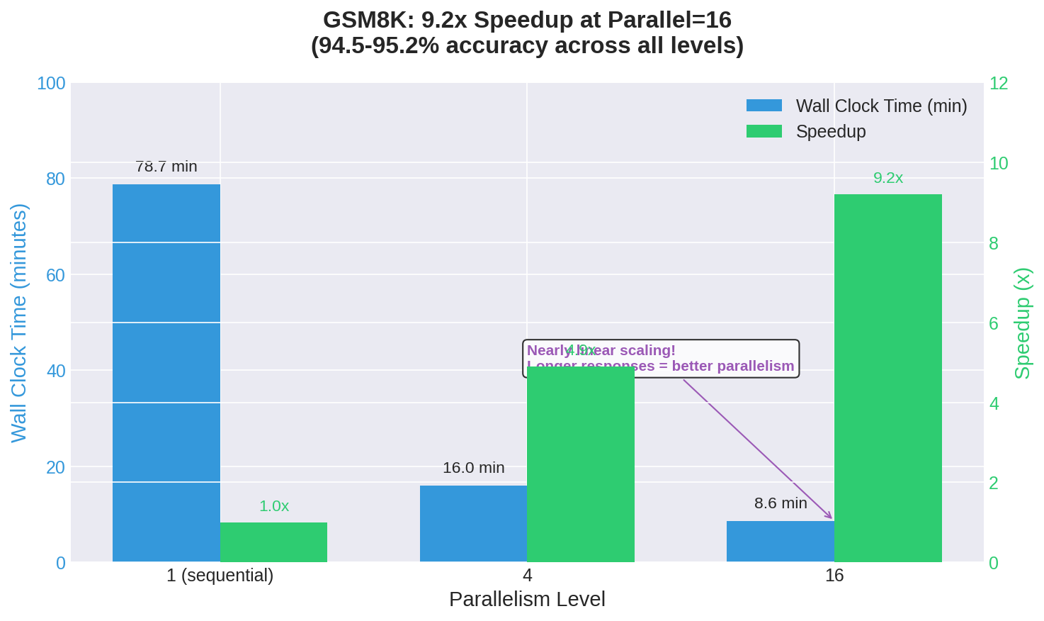
| Parallelism | Accuracy | Avg Time/Question | Wall Clock Time | Speedup |
|---|---|---|---|---|
| 1 | 95.2% | 3.58s | 78.7 min | baseline |
| 4 | 94.5% | 1.75s | 16.0 min | 4.9x |
| 16 | 95.1% | 2.43s | 8.6 min | 9.2x |
GSM8K shows even more dramatic scaling. The 9.2x speedup at parallel=16 approaches the theoretical maximum much more closely than MMLU did.
Why does GSM8K scale better? The answer lies in response length. MMLU questions generate short responses—often just a single letter with minimal reasoning. GSM8K requires step-by-step mathematical reasoning, generating hundreds of tokens per response.
Longer responses mean each request spends more time in the “generation” phase relative to the “setup” phase. vLLM’s continuous batching is most efficient during generation, where multiple sequences can share the same forward pass through the model. Short responses spend proportionally more time on per-request overhead that can’t be parallelized.
The accuracy variation (94.5% to 95.2%) is slightly larger than MMLU but still within normal statistical noise for a 1,319-question benchmark. There’s no evidence that concurrent processing degrades math reasoning quality.
A note on reproducibility: even with temperature set to 0.0 (greedy decoding), results aren’t perfectly deterministic. GPU floating-point operations accumulate in non-deterministic order, and when two tokens have nearly identical logits, tiny rounding differences can flip the decision. The ~0.5% variation we observe represents roughly 30-60 questions out of 14,042 where the model is genuinely uncertain and floating-point noise tips the balance. True determinism requires sacrificing performance—deterministic CUDA algorithms are significantly slower. For benchmarking purposes, this variation is small enough to treat as noise.
What’s Actually Happening Inside vLLM
When you send parallel requests to vLLM, several things happen:
-
Request queuing: Incoming requests are held in a queue until the inference engine is ready to process them.
-
Dynamic batching: vLLM groups queued requests into batches that can be processed together. Unlike static batching (which waits for N requests before starting), continuous batching adds new requests to an in-progress batch as slots become available.
-
Shared forward passes: During token generation, all active sequences share the same model forward pass. The GPU processes a batch of tokens across all sequences simultaneously.
-
Variable completion: As sequences finish (by hitting their stop token or max length), their slots are freed for new requests from the queue.
This architecture means that parallelism doesn’t require waiting for batch boundaries. A request that arrives while 15 others are being processed can join the next forward pass immediately, rather than waiting for all 15 to complete.
The overhead you do see—the reason parallel=16 isn’t 16x faster—comes from several sources:
- Memory bandwidth: Moving more data between GPU memory and compute units
- Attention computation: Each sequence’s key-value cache must be accessed during attention layers
- Scheduling overhead: Managing which sequences get which slots in each batch
For most workloads, these overheads are small compared to the compute time saved by parallel processing.
Practical Implications
For batch processing: Always use parallelism. If you’re processing a dataset overnight, there’s no reason to run sequentially. Parallel=16 or higher will dramatically reduce your total runtime with no accuracy penalty.
For latency-sensitive applications: There’s a trade-off. At parallel=16, individual request latency increases (0.030s → 0.101s for MMLU). If you need sub-50ms responses, high parallelism will hurt. If you can tolerate 100ms responses, parallelism lets you serve more users simultaneously.
For cost optimization: On cloud GPU instances, you’re paying by the hour. Processing 5x faster means paying for 5x fewer hours. The parallel=16 configuration that took 1.5 minutes for MMLU would have taken 7.1 minutes sequentially—nearly 5x the GPU time.
For capacity planning: If your production system handles N requests per second with sequential processing, it can handle roughly 5-9N requests per second with aggressive batching (depending on response length). That’s a significant multiplier before you need to scale horizontally.
The Sweet Spot
For the Qwen3-VL-30B model on this hardware:
- Parallel=4 offers a good balance: 2.5-4.9x speedup with minimal increase in per-request latency
- Parallel=16 maximizes throughput but individual requests take 3-5x longer
- Beyond 16 likely shows diminishing returns as GPU memory becomes the bottleneck
The optimal parallelism depends on your workload. For batch jobs, go as high as memory allows. For interactive applications, start with parallel=4 and tune based on your latency requirements.
One More Data Point
While running these benchmarks, I also completed the GSM8K tests for the 11 model configurations that were missing math results. That data will be integrated into the consolidated results, but the key finding from the parallelism experiment stands on its own: if you’re using vLLM and processing requests sequentially, you’re leaving 4-9x performance on the table.
The space heater continues its work. The benchmarks continue their march through model after model. And the data continues to reveal that the “obvious” way of doing things—one request at a time, bigger models are always better, quantization always hurts—often isn’t optimal at all.
This is Part 4 of a 5-part series. Part 5 wraps up with a practical decision chart for choosing the right model.